What is Data Validation?

The data validation feature in Excel can be very useful when creating forms or reports. It helps you to control what can be entered by a user in your worksheet or template. For instance you can create dropdown menus within a cell, restrict data entry such as text length as well as create custom rules containing various functions.

Creating a dropdown menu:

To create a dropdown list in Excel, the first thing you will need to do is name your list of items. Then that named list will be used as the source for the Data Validation dropdown menu.

To create a named range:

• Create the list as shown below
• Highlight the range A1:A5 (include the heading)
• Click on the Formulas tab

• From this tab select the Create from Selection command button.
• A dialog box appears containing a number of options.
• Select the option Top row (doing this will create the name from the value found at the top of the list).
  Note: the name created is Project_Status with an underscore as named ranges can’t contain spaces.

Data Validation

Now that you have created a named range, you can use that to create a dropdown menu in Excel.

• Select the cells you want to apply the data validation to (this maybe on a new sheet)

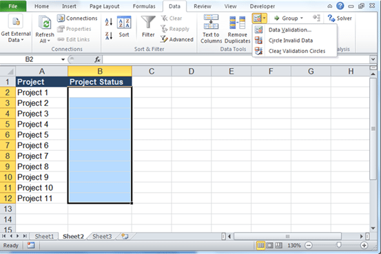
• On the Data tab, click Data
  Validation.
• From the dropdown list under Allow: select the option List as shown below.

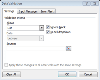
• In the Source: box type an equals sign and then the named range e.g. =Project_Status or you can also press the F3 function key and select the named range.

• Click OK to close the dialog box.
• Try it out in the your worksheet:

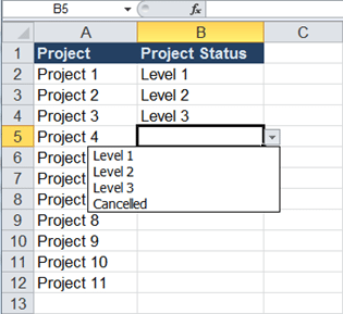
Now the best part, combining the above list with conditional formatting to achieve out desired result. For example when a user selects Cancelled from the dropdown list you may want it to change to red or if the user selects Level 1 you may want that option to turn blue.

What is Conditional Formatting?

With conditional formatting, you can select one or more cells, and create various rules for how those cells are formatted. If the rules that you create are met, then the formatting will be applied to the highlighted cells.

Applying Conditional Formatting to your dropdown menu

You are now going to setup conditional formats so that a cell:

• turns green if it contains the text Level 1 and
• turns red if it contains the text Cancelled

Follow these steps to apply conditional formatting to the cells B2:B12:

• Highlight the cells to be formatted.
• On the Home tab, click on Conditional Formatting

• To format the text Level 1, click on Highlight Cell Rules, then select Equal To…
• Type the text Level 1 as shown below:

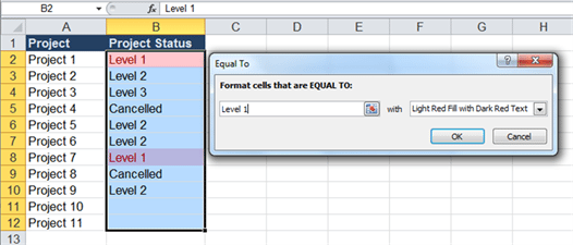
• From the right hand side select a format or create a custom format.

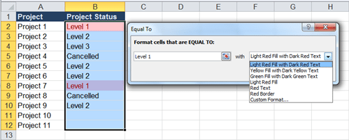
• In your case select the option Green Fill with Dark Green Text
• Click OK

2nd Conditional Format

To colour all the cells containing Cancelled in red, you can apply a second conditional format to the cells.

• Highlight the cells to be formatted, B2:B12.
• On the Home tab, click on Conditional Formatting

• To format the text Cancelled, click on Highlight Cell Rules, then select Equal To…
• Type the text Cancelled.

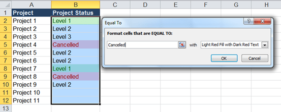
• From the right hand side select a format or create a custom format of your own.

• In your case select the option Light Red Fill with Dark Red Text.
• Click OK

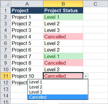
Now you have combined the conditional formatting feature with Data Validation in Excel.

If so desired you can create more conditional formats for the rest of the Project Level options. For example, Level 2 could be Light Blue Fill with Dark Blue Text (note: change this using Custom Format…)

Hope this gives you a taste for what you can do with the many different features available within excel, when you start to combine them.